(This Spring 2015 handout is the main one of the lecture, so worth posting separately. Some formatting has been challenged in the post to the web. It's also found here.)
These are basic tips for Excel that many experienced users may already know. That said, I know sometimes the simplest things can be frustrating when you don’t know how to do it, so that’s the genesis of this document. Almost all of these tips are much easier to show on a screen than to explain in text, so don’t be shy in asking to see these in action.
Column widths
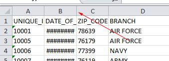
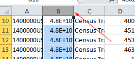
Sometimes you’ll see a weird exponent number or ##### or a instead of a number or date you expect:
Excel is telling you it can’t show you the whole number or date because the column isn’t wide enough.
- Move your cursor to the right dividing line between the two columns right between the column letters until you see your cursor change to a line with two arrows going right and left. Click and drag the column wider.
- If you do that same thing but double-click on the line, it will change the width of the column to fit the longest content.
- Or, click on the triangle that is to the left of the A column and above the number 1 row, which will select everything in the sheet. Then move your cursor to the right dividing line between two columns and double-click to widen all the columns to their maximum width.
- Right click on any of the column letters and select “column width” from the pop-up window. You can then enter a character width for all the columns. (If you have more than one or all columns selected, it will change them all.)
Freezing rows and columns
 Sometimes you need to scroll further into a file, but don’t know what the columns and rows mean anymore because they are stuck at the top and left of the file. It’s easy to “Freeze Panes” in Excel so you can carry those descriptions with your scroll.
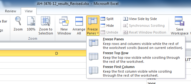
 - In many cases, you just want to freeze the top row or first column, and there are special menu items there under the View ribbon to Freeze Panes for that.
- If you want to freeze more than the top row, put cursor in the cell furthest to the top and left that you still want to move, and then choose View > Freeze Panes > Freeze Panes. This will freeze anything to the top and left of that cell.
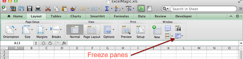
- To unfreeze panes, you can find it under View > Freeze Panes. (On Mac: Layout ribbon > Window group > Freeze Panes
Filtering
 One of the most useful things Excel can do is to filter your data so you only see what you want.
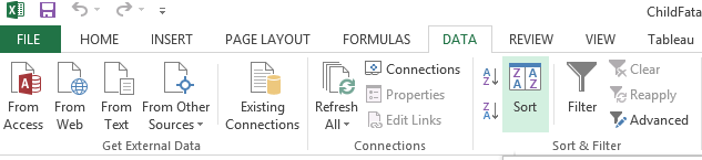
- Filter multiple columns: If you have a single cell selected, or all cells selected, and go to Data > Filter it will put the drop-down filter arrows on all the columns. You can then filter one column, then go to another column to further filter the rows.
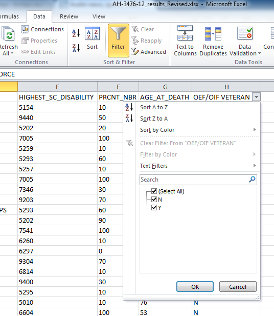
- Filter a single column: Click on the column letter to choose the column. Go to the Data ribbon to Filter, which puts a drop-down arrow for your column. Click on the arrow to get a list of all the unique fields in your column. You can choose which ones you want to see.
Sorting
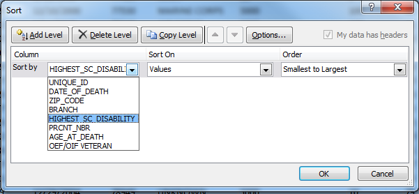 Equally useful is to sort your data on one or more columns. You can sort all your data or just a selection. (But be very careful you aren’t sorting such a small portion that you mess up your data. Always choose entire rows.)
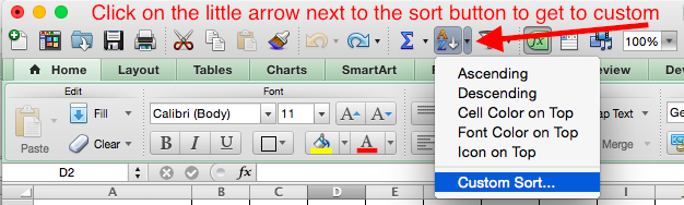
 - Select all or some rows of your data, then go under the Data ribbon to Sort so you get the sort wizard. If your data has headers and the box is checked, the “Sort by” column should show your headers.
- You can add levels, so you can sort by City, then Last Name within each City.
Copying cells
Magical copy point
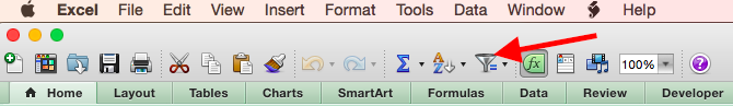
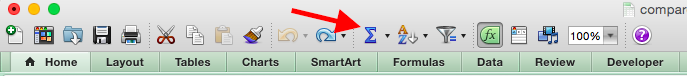
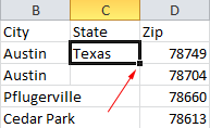 There are too many ways to copy date in Excel to list them all, but here are some useful tidbits. There is a magical handle in a selected cell that allows you to copy that content in different ways. Put your cursor on the lower-right-hand dot of the selected arrow (see the arrow at right) and your cursor will become a thin black plus sign (as opposed to a thick white one.)
- When on the magical copy point, you can click and drag along other cells and it will copy the cell into the highlighted sections
- If you double-click the magical copy point, the cells below will be filled with the content, for a long as there are filled adjacent cells.
- If you highlight two sequential numbers and copy to other cells (either method) it will try to keep up the same number sequence. So a cell with 1 and an adjacent cell with 2 will copy into further cells as 3, 4, 5 and so on.
Other copying tips
- If you have multiple cells in your clipboard, you must select the same number of cells into which to copy. Or, you can copy multiple cells into a single cell and the data will “fan out” into adjoining cells. Be careful you don’t overwrite other data!
- Watch that sequential numbers. If you use the magical copy point on ZIP codes, it may try to make new numbers that are sequential!
- You can copy filtered and sorted data into a new sheet to work on just that data without affecting the original data.
Multiple windows
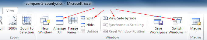
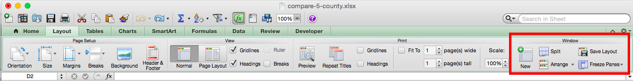
It can be frustrating working on multiple files as once if you don’t know how to “show” them at the same time. All the tools you need are on the View ribbon. (Mac: Layout ribbon > Window group.)
- Click on Arrange All to resize all your windows so you can see them all. You’ll get to choose how to stack them.
- Split screen allows you to windows into the same file, so you can see the top and bottom at the same time without scrolling. Don’t get confused!
- View Side by Side allows you to look at two files at once, scrolling them together if you wish. Very useful for comparing two files.
- Switch windows simply allows you to choose another open file and bring it to the front so you can see it. (Mac: main Window menu.)
Data warning: What are the green triangles!
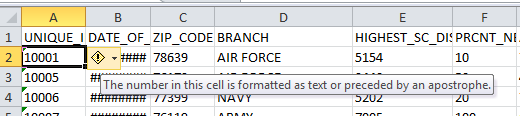
Green triangles mean Excel is telling you the *MAY* be a problem with your data. Getting the green triangle does not guarantee there is a problem. Excel is just noting that something isn’t following a pattern or isn’t formatted as expected. To see what the warning is, select the cell, and then hover over the exclamation point. You can choose the little arrow to make suggested corrections, if needed. Some common problems:
- Numbers are stored at text. Sometimes you want numbers as text, so this might be OK.
- Adjacent formulas don’t fit the same pattern. If you have a column of percentages, and then one of the cells doesn’t follow a logical pattern (you might have a total), then Excel let’s you know there may be something amiss.
In short, let the green triangles show you where to check for problems, but be confident when you are purposefully breaking a pattern.
Opening a .txt or .csv file
Sources will often send data that isn’t in an Excel file. If you open it in Word, it’s crazy, but Excel can do some good stuff with this, especially fixed-column data.
Importing delimited files
 .csv stands for Comma Separated Value, which means the file is really like a spreadsheet, but they used commas or something similar to divide the lines of text into rows. Excel is great with these.
- Launch Excel, and then go under the File ribbon to Open and then find your file. (Sometimes you have to change the File Type down by the Open button to “All Files” to see your text file.)
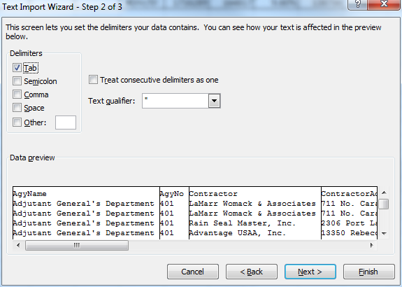
- You’ll get the Text Import Wizard. If you are opening a CSV file, you’ll want to choose “Delimited” on the first screen.
- At the next screen you can choose which character is creating the columns. If Tab doesn’t separate the columns like you see above, then uncheck it and try Comma. If it’s anything other than those two, usually your source can tell you what the delimiter is. (Or it might be a fixed-width file, which is handled below.)
- Once you find the right delimiter, go to the next screen. Click on each column and see what “column data format” that Excel suggests, and change it if it is obviously wrong. General is fine for both text and numbers. Dates are the most common changes.
- Click Finish and you should be looking at a spreadsheet of nice, neat rows. If not, start over and try different settings.
Importing fixed-width files
 Some systems spit out data using spaces to create columns of text. Excel can turn these into spreadsheets, too.
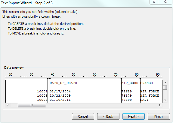
- Open the file from Excel. The first screen may guess that it is a fixed-width file, but you can guess by the preview as well.
- On the next screen is where you choose to create columns. You can click on an existing break line to move it to the right or left as you see fit in the preview. You can click anywhere in the preview window to add a new break line, or double-click on one to remove it. Make sure you check all across the width of the file.
- The Next screen is much like above, where you choose what the data format should be for each column.
- Once you finish, you may have some cleanup to do, but you’ll be a lot further ahead than using a regular text editor!
Insert anything
The secret to inserting anything (cell, column, comment) is usually to right-click.
- Insert a column by right-clicking to the column to the right of it and choosing insert.
- If you have text in your clipboard, it will paste that into the created column.
- If you select more than one column and then right-click to insert, then you’ll add the same number of columns.
- To insert a row, right-click on the row header and choose insert.
- If you want to insert more than one row, select the same number of rows below, then right-click to insert.
- To insert cells, right-click and choose insert. You’ll be asked how to move the other cells affected. BE CAREFUL not to screw up your data by shifting it incorrectly.
- To insert a worksheet, click on the little tab with the starburst next to the last named worksheet at the bottom of the screen.
- There are all kinds of special insert stuff under the Insert ribbon.
 Simple Sums
 Formulas are why Excel was invented. Who wants to do math? There can be a multi-day class on formulas alone, so this covers just two things: AutoSum and Percentages.
AutoSum
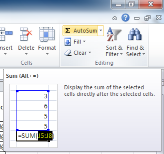
- On the Home ribbon is AutoSum. If you put your cursor in a cell at the bottom of a row of number and press AutoSum, Excel will guess which cells you want to add. You’ll know which ones as Excel highlights them for you.
- If it doesn’t guess right, you can click first on the top cell, then the bottom cell, and it will adjust the highlight.
- You can always adjust the formula in the Formula Bar, but again, that’s another class.
- =SUM(J5:J8) will add all cells in between J5 and J8 together. =SUM(J5,J8) will add just the two cells together.
Percentage (typing a formula!)
- Put your cursor in the cell you want the percentage to be in. Begin typing =SUM and you’ll see that Excel wants to help you type it. Get to =SUM( and then click in the cell of the top number in your division, then type in the slash / and then click on the denominator, or what you are dividing by. Then close the parenthesis. So it should look something like this:
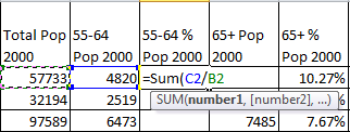
=SUM(C2/B2)
You’ll end up with a decimal number that you have to turn into a percentage. Right-click on the cell and you’ll get a pop-up menu. Choose Format Cell, then under the Number tab, choose Percentage and pick what decimal places you want to use.
- There are some tricks to clicking around the cells to add the right numbers for the formula. If it throws you for a loop, hit the Esc key to start over. Or, just type in the column and row by hand.
Making charts in Excel
Some day I may add more detail to this on making charts in Excel, but there are also plenty of references out on the web:
Using Google Spreadsheets
Everything worth doing in Excel can be done in Google Spreadsheets, which is free and supports collaborative editing. Only downside is the need for Internet access.
