QGIS: Save to KML

QGIS is free, open source, multi-platform. Download at qgis.org. It has lots of prerequisites, so be patient and methodical.

For this exercise, we are opening a file with all counties in Texas, then selecting the five in our MSA (Travis, Williamson, Hays, Bastrop, Caldwell) and saving them out separately as its own KML file.

This is a QGIS lesson on how to convert a .shp file to .kml to be used with Fusion Tables.

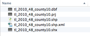
Download the zip file tl_2010_48_county10.zip. Unzip the file so you have a folder of contents. Note there are five files, including one .shp

In QGIS, go to Layer > Add Vector Layer. (Or look for the icon at left.)  Browse to your .shp file. 

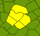
Use the selection tool (pictured at left) to select Travis county, then hold the Command key (Mac) and select on Bastrop, Caldwell, Hays and Williamson counties. This should allow you to add them to your selection. It will look something like the photo at right, through your colors may be different, since QGIS picks them at random.

In the layers panel at left, right-click on the layer and choose Save Selection As ...

Click on the Format option and then change the format option to "Keyhole Markup Language (KML).

Next, you need to choose where to save the file, and what to name it. Under Save As, click the Browse button, name your file in the Save As window what you want to name it, then negotiate to the folder where you want to save your file. Click "Save" to set the settings.

Then you'll need to check your CRS, or Coordinate Reference System. I've been OK using the NAD83:4269 setting, though I've seen some references suggest that Google wants WGS84:4269. Type the number into the Filter field and you'll see your's listed. Choose the one in the bottom window.

Once all of those are set, you can hit OK on the "Save vector layer as" window, and your new KML file will be saved. It is that new AustinMSACounties file that you can upload into Google Fusion Tables.

Categories: Handouts, QGIS, Spring 2014

GIS programs: Quantum GIS

This class period covered from background on GIS theory, projections, shapefiles and more, and served as the introduction to several classes focusing on using Quantum GIS.

(Yes, I know this post needs more detail. For now, it's just links to the presentation and data.)

Presentation

The files used:

• APD Districts
• CasesWSubjectUnderInfluence.csv
• CasesWSubjectUnderInfluence.csvt
• uof-reports.csv
• uof-reports.csvt

Categories: Assignments, QGIS, Spring 2013

Clipping shapefiles in QGIS

This next assignment focuses on using QGIS to clip one shapefile with the selection of another, and also to join a shapefile with a .csv data file in QGIS.

Goal: To make a make a map in QGIS that shows ACS data for a zip codes within a particular county. It's fairly complicated, but here are the overall steps:

• Download shapefiles for the county and the zip codes.
• Clip the zip codes file to include only those for the county you care about.
• Download the ACS data and clean it up for your purposes, then save it as a csv file.
• Create a csvt file to define the columns so QGIS understands them.
• Join the ACS data to the modified shapefile.
• Style the map so you can see the variance in desired data.

Now for some detail:

THE SHAPEFILES

• Work on the shapefiles first. Download the shapefile for ZIP Code Tabulation Areas for your state. (2010 data is fine). Same for County (and equivalent). You can find them at the Census Bureau's Tiger/Line site.:
• Open the Counties file and then the Zip Code file. Move the Zips on top so and change the properties of the layer so it is transparent and you can see the counties underneath.
• Open the Attribute Table for the Counties file and use the search to find your county. (You might want to click the “Show selected Only” box.) Close that attribute window
• Now your county is selected. You can go to Vector > Geoprocessing Tools > Clip. Remember to cut up, so the Zips are on top. Use only the “selected feature” from the county layer. You’ll need to browse to where you want the file and name it. Do it. Go ahead and add the layer to your workbook.
• Now you have zip codes for only your county! You can remove the other layers.

THE DATA

• Go to the American Factfinder.
• Go to the advanced search. Set your geography to 5-digit Zip code Tabulation area in Texas.
• Find a table you are interested in. You might stick with ACS-5-year data to have good ZIP code data. I’d allow 2010 Census if you desire. (Geographic mobility is one worth looking at.) Look at the detail page to make sure it has data you are interested in, but ...
• Download the table from the search results page. It is important to do it there instead of in the detail page.
• Open up the.metadata.csv file and look at the description of the data. Take note of the column names of the data you want. You’ll want both the EST (Estimate) fields and the MOE (Margin of Error) fields.
• Open up your “with_ann.csv” file and delete the columns you don’t need.
• Open up TextEdit and create a text file that describes what each kind of column is in your date. (Refer to this post for more details on CSVT: ). A couple of notes: The ZIP code, GEOid and any other column you will JOIN on need to be “String”. Number columns you want to act on with shading need to be “Integer” or “Real”. Name this file the same as your data, except “.txt”.
• Find the file on your desktop and right-click on it and do Get Info. Under "Name and Extension" change the file name from .txt to .csvt. When you close it, the computer will ask you if you want to keep .txt or use .csvt. Tell it to use .csvt.

THE JOIN

• Add the CSV file to your QGIS document using Add Vector Layer. Open the properties of the shapefile and use the Join tab to match your fields.
• Now change the Style of your shapefile to show your colors.

You are done! At least with analysis.

To publish online, you want to do a Save As on the layer and save it as KML to upload to fusion tables.

To print requires a whole different lesson believe it or not.

Categories: Assignments, QGIS, Spring 2013